Adler plotting utilities
For ease of use Adler provides helper functions which can be used to make common solar system object plots, such as light curves and phase curves.
[1]:
from adler.objectdata.AdlerPlanetoid import AdlerPlanetoid
from adler.science.PhaseCurve import PhaseCurve
from adler.utilities.plotting_utilities import plot_errorbar

import numpy as np
import matplotlib.pyplot as plt
import matplotlib.gridspec as gridspec
import astropy.units as u
[2]:
# retrieve the object data
ssoid = "8268570668335894776"
fname = "../../notebooks/gen_test_data/adler_demo_testing_database.db"
planetoid = AdlerPlanetoid.construct_from_SQL(ssoid, sql_filename=fname)
No observations found in u filter for this object. Skipping this filter.
No observations found in y filter for this object. Skipping this filter.
n unpopulated in MPCORB table for this object. Storing NaN instead.
uncertaintyParameter unpopulated in MPCORB table for this object. Storing NaN instead.
[3]:
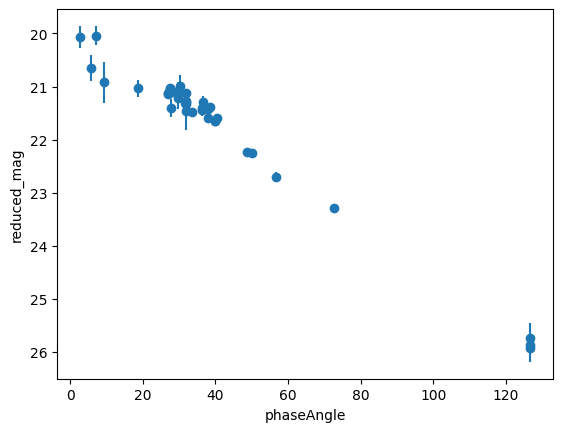
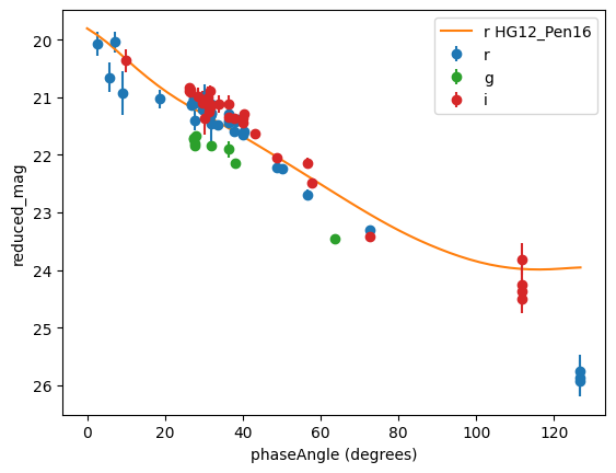
# use the adler plotting function to create a phase curve from the planetoid object
fig = plot_errorbar(planetoid, filt_list=["r"])
[4]:
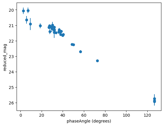
# with matplotlib we can access axes properties and update them after the fact

# ax1.__dict__
[5]:
# access the axes object to update attributes
ax1 = fig.axes[0]
ax1.set_xlabel("phaseAngle (degrees)")
[5]:
Text(0.5, 24.0, 'phaseAngle (degrees)')
[6]:
# replot the figure
fig
[6]:
[7]:
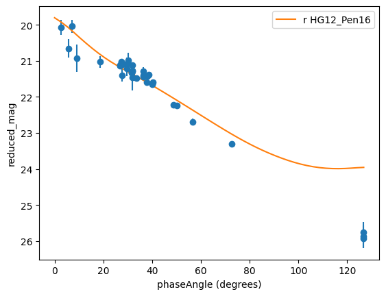
# fit a phase curve model to the data

filt = "r"
sso = planetoid.SSObject_in_filter(filt)
obs = planetoid.observations_in_filter(filt)

H = sso.H
G12 = sso.G12

pc = PhaseCurve(H=H * u.mag, phase_parameter_1=G12, model_name="HG12_Pen16")
alpha = np.linspace(0, np.amax(obs.phaseAngle)) * u.deg
red_mag = pc.ReducedMag(alpha)
/home/docs/checkouts/readthedocs.org/user_builds/adler/envs/latest/lib/python3.10/site-packages/sbpy/photometry/iau.py:53: InvalidPhaseFunctionWarning: G12 parameter could result in an invalid phsae function
  warnings.warn(msg, exception)
[8]:
# add this phase curve to the figure
ax1.plot(alpha.value, pc.ReducedMag(alpha).value, label="{} {}".format(filt, pc.model_name))
ax1.legend()  # udpate the figure legend
[8]:
<matplotlib.legend.Legend at 0x75c1c4df74f0>
[9]:
fig
[9]:
[10]:
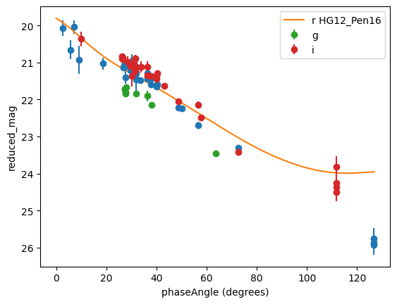
# we can also pass the fig object to the plotting function again to add more data
fig2 = plot_errorbar(planetoid, fig=fig, filt_list=["g", "i"], label_list=["g", "i"])

# update the legend
ax1 = fig2.axes[0]
ax1.legend()
[10]:
<matplotlib.legend.Legend at 0x75c192688f10>
[11]:
fig2
[11]:
[12]:
# inspect the different items that have been plotted
[13]:
ax1._children
[13]:
[<matplotlib.lines.Line2D at 0x75c19288c220>,
 <matplotlib.collections.LineCollection at 0x75c19288c3a0>,
 <matplotlib.lines.Line2D at 0x75c192688b20>,
 <matplotlib.lines.Line2D at 0x75c1926d5ff0>,
 <matplotlib.collections.LineCollection at 0x75c1926d71c0>,
 <matplotlib.lines.Line2D at 0x75c1927241f0>,
 <matplotlib.collections.LineCollection at 0x75c1927242e0>]
[14]:
ax1.containers
[14]:
[<ErrorbarContainer object of 3 artists>,
 <ErrorbarContainer object of 3 artists>,
 <ErrorbarContainer object of 3 artists>]
[15]:
# add the legend label to the r filter data
ax1.containers[0]._label = "r"
ax1.legend()
[15]:
<matplotlib.legend.Legend at 0x75c192688220>
[16]:
fig2
[16]:

[17]:
# we use `plot_errorbar` to save the figure, without adding anything extra to the figure
fig3 = plot_errorbar(planetoid, fig=fig2, filename="phase_curve_{}.png".format(ssoid))
[18]:
fig3
[18]:
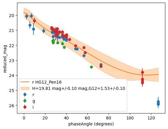
[19]:
# if the PhaseCurve model has uncertainties we can display the range of possible values
pc.H_err = 0.1 * u.mag
pc.phase_parameter_1_err = 0.1
pc_bounds = pc.ReducedMagBounds(alpha, 3)
[20]:
# helper function to return PhaseCurve parameters as a string
l = pc.ReturnParamStr(err=True)
l
[20]:
'H=19.81 mag+/-0.10 mag,G12=1.53+/-0.10'
[21]:
ax1 = fig3.gca()
ax1.fill_between(
    alpha.to_value(),
    pc_bounds["mag_min"].to_value(),
    pc_bounds["mag_max"].to_value(),
    color="C1",
    alpha=0.3,
    label=l,
)
ax1.legend()
fig3
[21]:
[ ]: