Adler colour measurement

Adler includes a function col_obs_ref which calculates the difference between the most recent brightness data point in the observation (obs) filter and a number of previous measurements in the reference (ref) filter.

from adler.objectdata.AdlerPlanetoid import AdlerPlanetoid
from adler.objectdata.AdlerData import AdlerData
from adler.science.PhaseCurve import PhaseCurve
from adler.science.Colour import col_obs_ref
from adler.utilities.plotting_utilities import plot_errorbar
from adler.utilities.science_utilities import apparition_gap_finder, get_df_obs_filt

import numpy as np
import pandas as pd
import matplotlib.pyplot as plt
import matplotlib.gridspec as gridspec
import astropy.units as u

# ssObjectId of object to analyse
ssoid = "6098332225018"  # good MBA test object

# retrieve the object data
fname = "../../notebooks/gen_test_data/adler_demo_testing_database.db"
planetoid = AdlerPlanetoid.construct_from_SQL(ssoid, sql_filename=fname)

No observations found in u filter for this object. Skipping this filter.
No observations found in y filter for this object. Skipping this filter.
n unpopulated in MPCORB table for this object. Storing NaN instead.
uncertaintyParameter unpopulated in MPCORB table for this object. Storing NaN instead.

# check orbit parameters
e = planetoid.MPCORB.e
incl = planetoid.MPCORB.incl
q = planetoid.MPCORB.q
a = q / (1.0 - e)
Q = a * (1.0 + e)
print(a, e, incl)

3.1637750412330092 0.13967823750326572 4.440569999999986

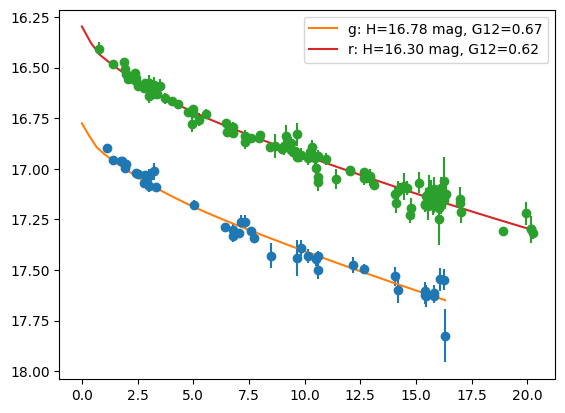
# plot and fit the phase curves in g and r filters

fig = plt.figure()
gs = gridspec.GridSpec(1, 1)
ax1 = plt.subplot(gs[0, 0])

adler_data = AdlerData(ssoid, planetoid.filter_list)

for filt in ["g", "r"]:
    # get observations and define a phase curve model to fit
    sso = planetoid.SSObject_in_filter(filt)
    obs = planetoid.observations_in_filter(filt)

    H = sso.H
    G12 = sso.G12
    pc = PhaseCurve(H=H * u.mag, phase_parameter_1=G12, model_name="HG12_Pen16")

    alpha = np.linspace(0, np.amax(obs.phaseAngle)) * u.deg

    pc_fit = pc.FitModel(
        np.array(getattr(obs, "phaseAngle")) * u.deg,
        np.array(getattr(obs, "reduced_mag")) * u.mag,
    )
    pc = pc.InitModelSbpy(pc_fit)
    red_mag = pc.ReducedMag(alpha)

    adler_data.populate_phase_parameters(filt, **pc.ReturnModelDict())

    # add this phase curve to the figure using the Adler plotting function
    fig = plot_errorbar(planetoid, filt_list=[filt], fig=fig)
    ax1 = fig.axes[0]
    ax1.plot(
        alpha.value,
        pc.ReducedMag(alpha).value,
        label="{}: H={:.2f}, G12={:.2f}".format(filt, pc.H, pc.phase_parameter_1),
    )
    ax1.legend()

ax1.invert_yaxis()

plt.show()

Input model name HG12_Pen16 does not match model name  in AdlerData. Parameters will be overwritten.
Input model name HG12_Pen16 does not match model name  in AdlerData. Parameters will be overwritten.

# inspect the r filter phase curve model
adler_data.get_phase_parameters_in_filter("r", "HG12_Pen16").__dict__

{'filter_name': 'r',
 'phaseAngle_min': nan,
 'phaseAngle_range': nan,
 'observationTime_max': nan,
 'nobs': 0,
 'arc': nan,
 'n_outliers': 0,
 'n_std_outliers': 0,
 'sustained_outliers': nan,
 'model_name': 'HG12_Pen16',
 'H': <Quantity 16.29653482 mag>,
 'H_err': <Quantity 0.00515468 mag>,
 'phase_parameter_1': np.float64(0.6201164104813285),
 'phase_parameter_1_err': np.float64(0.037407505577815164),
 'phase_parameter_2': None,
 'phase_parameter_2_err': None}

# inspect the g filter phase curve model
adler_data.get_phase_parameters_in_filter("g", "HG12_Pen16").__dict__

{'filter_name': 'g',
 'phaseAngle_min': nan,
 'phaseAngle_range': nan,
 'observationTime_max': nan,
 'nobs': 0,
 'arc': nan,
 'n_outliers': 0,
 'n_std_outliers': 0,
 'sustained_outliers': nan,
 'model_name': 'HG12_Pen16',
 'H': <Quantity 16.7755294 mag>,
 'H_err': <Quantity 0.01306086 mag>,
 'phase_parameter_1': np.float64(0.6711101977751897),
 'phase_parameter_1_err': np.float64(0.08615904379646462),
 'phase_parameter_2': None,
 'phase_parameter_2_err': None}

Determine the apparitions (periods of observability) of the object.

Get the boundary times for each apparation of the object in the survey using the Adler helper function apparition_gap_finder. In this example we will just look at changes in colour for a single apparition

# combine all measurements in r and g into one dataframe as apparitions are filter independent
df_obs_all = pd.DataFrame()
for filt in ["r", "g"]:
    obs = planetoid.observations_in_filter(filt)
    _df_obs = pd.DataFrame(obs.__dict__)
    df_obs_all = pd.concat([df_obs_all, _df_obs])
df_obs_all = df_obs_all.sort_values("midPointMjdTai")

# get the boundary times
t_app = apparition_gap_finder(np.array(df_obs_all["midPointMjdTai"]))
print(t_app)

[60231.19309 60666.23231 61120.35642 61469.38552 61939.36191 62442.20849
 62883.29148 63305.32256 63744.27944 63951.09539]

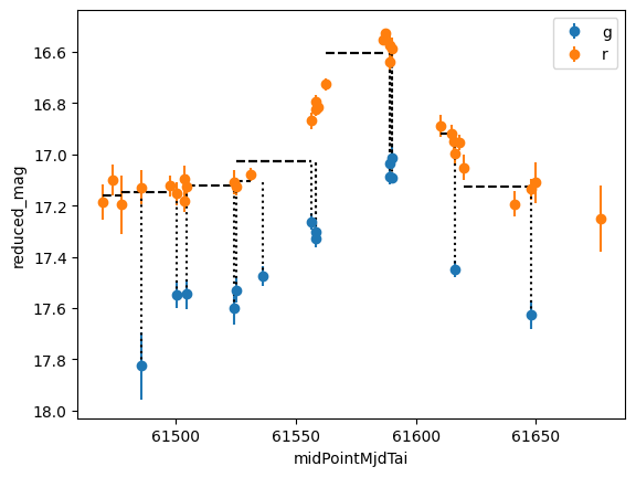
Now we can inpsect how the colour of the object varies (or not) as a function of time. The adler function col_obs_ref will compare the latest observation in a given filter with observations in another filter. By setting parameter N_ref one can set how many past obsevrations to use when calculating the latest colour.

Here we simulate observations coming night-by-night and the calculation of a g-r colour for the object

# define colour function parameters

# set number of reference observations to use for colour estimate, there are multiple options
# N_ref = 5
N_ref = 3
# N_ref = 1
# N_ref = None # selecting None uses all previous reference filter measurements

# observation and filter field names
x_plot = "midPointMjdTai"  # time column
y_plot = "reduced_mag"  # magnitude column
yerr_plot = "magErr"  # magnitude uncertainty column
filt_obs = "g"  # observation filter
filt_ref = "r"  # reference filter (we are calculating a filt_obs - filt_ref colour)

# define colour field names
colour = "{}-{}".format(filt_obs, filt_ref)
colErr = "{}-{}Err".format(filt_obs, filt_ref)
delta_t_col = "delta_t_{}".format(colour)
y_ref_col = "{}_{}".format(y_plot, filt_ref)
x1_ref_col = "{}1_{}".format(x_plot, filt_ref)
x2_ref_col = "{}2_{}".format(x_plot, filt_ref)

fig = plt.figure()
gs = gridspec.GridSpec(1, 1)
ax1 = plt.subplot(gs[0, 0])

col_dict_list = []
for app_i in range(len(t_app) - 1):
    # consider only one apparition
    if app_i != 3:
        continue

    time_min = t_app[app_i]
    time_max = t_app[app_i + 1]

    _df_obs_all = df_obs_all[
        (df_obs_all["midPointMjdTai"] >= time_min) & (df_obs_all["midPointMjdTai"] < time_max)
    ]
    _time_max = np.amax(_df_obs_all["midPointMjdTai"])

    # get the phase curve model and observations for each filter

    # get the stored AdlerData parameters for the observation filter
    ad_g = adler_data.get_phase_parameters_in_filter(filt_obs, "HG12_Pen16")
    pc_g = PhaseCurve().InitModelDict(ad_g.__dict__)  # make the PhaseCurve object from AdlerData
    # get the phase curve model for the reference filter
    ad_r = adler_data.get_phase_parameters_in_filter(filt_ref, "HG12_Pen16")
    pc_r = PhaseCurve().InitModelDict(ad_r.__dict__)
    # get the observations in both filters
    df_obs = get_df_obs_filt(
        planetoid, filt_obs, x1=time_min, x2=_time_max, col_list=[y_plot, yerr_plot], pc_model=pc_g
    )
    df_obs_ref = get_df_obs_filt(
        planetoid, filt_ref, x1=time_min, x2=_time_max, col_list=[y_plot, yerr_plot], pc_model=pc_r
    )

    ax1.errorbar(df_obs[x_plot], df_obs[y_plot], df_obs[yerr_plot], fmt="o", label=filt_obs)
    ax1.errorbar(df_obs_ref[x_plot], df_obs_ref[y_plot], df_obs_ref[yerr_plot], fmt="o", label=filt_ref)

    # simulate stepping through each new filt_obs observation
    x1 = time_min
    for xi in range(len(df_obs)):
        x2 = df_obs.iloc[xi][x_plot]

        # run the colour finding function here
        col_dict = col_obs_ref(
            planetoid,
            adler_data,
            filt_obs=filt_obs,
            filt_ref=filt_ref,
            N_ref=N_ref,
            x_col=x_plot,
            y_col=y_plot,
            yerr_col=yerr_plot,
            x1=x1,
            x2=x2,
        )
        col_dict_list.append(col_dict)

        # plot some lines to show the colour and mean reference
        ax1.vlines(df_obs.iloc[xi][x_plot], df_obs.iloc[xi][y_plot], col_dict[y_ref_col], color="k", ls=":")
        ax1.hlines(col_dict[y_ref_col], col_dict[x1_ref_col], col_dict[x2_ref_col], color="k", ls="--")

# store running colour parameters as a dataframe
df_col = pd.DataFrame(col_dict_list)
df_col = df_col.merge(df_obs, on=x_plot)

ax1.set_xlabel(x_plot)
ax1.set_ylabel(y_plot)
ax1.legend()
ax1.invert_yaxis()

plt.show()

# display the recorded colour parameters
df_col

	diaSourceId	midPointMjdTai	g-r	delta_t_g-r	g-rErr	reduced_mag_r	midPointMjdTai1_r	midPointMjdTai2_r	reduced_mag	magErr
0	5806484744413721495	61485.35880	0.664603	7.96148	0.138779	17.160866	61469.38552	61477.39732	17.825469	0.132
1	-1370847514993823225	61500.36601	0.399820	3.04185	0.061730	17.149109	61477.39732	61497.32416	17.548930	0.052
2	-6386483006798364737	61504.33885	0.413061	0.02451	0.067195	17.132855	61503.35033	61504.31434	17.545916	0.057
3	8031997375699514682	61524.28190	0.468237	19.96756	0.071485	17.132855	61503.35033	61504.31434	17.601093	0.062
4	7261031060333293464	61525.31814	0.410175	0.02461	0.047604	17.119983	61504.31434	61525.29353	17.530158	0.047
5	-2100995506165571482	61536.27685	0.369656	4.97307	0.043530	17.104826	61524.30740	61531.30378	17.474481	0.039
6	-4613899454603301440	61556.37692	0.237609	0.02406	0.116098	17.024827	61525.29353	61556.35286	17.262437	0.032
7	6671138127230663272	61558.20527	0.305192	1.85241	0.116098	17.024827	61525.29353	61556.35286	17.330019	0.032
8	-4138723505372602053	61558.20674	0.277199	1.85388	0.115563	17.024827	61525.29353	61556.35286	17.302026	0.030
9	1709187193968832045	61589.25295	0.483080	1.96801	0.092782	16.603103	61562.31723	61587.28494	17.086183	0.029
10	-8609372919476238181	61589.25519	0.432073	1.97025	0.094109	16.603103	61562.31723	61587.28494	17.035176	0.033
11	-796743135402922428	61590.00200	0.413271	0.02370	0.052214	16.599779	61589.27700	61589.97830	17.013050	0.044
12	8768036112299467593	61590.24357	0.491569	0.26527	0.035698	16.599779	61589.27700	61589.97830	17.091348	0.022
13	414337052068152629	61616.20243	0.529920	0.19328	0.041118	16.918264	61610.20336	61616.00915	17.448184	0.033
14	-8355039433456489093	61648.07405	0.500634	0.02498	0.080268	17.126752	61620.16575	61648.04907	17.627386	0.055

Now we can plot how the colour changes as a function of time

# find filt_obs - filt_ref of newest filt_obs observation to the mean of the previous N_ref filt_ref observations
# colour code by time diff between obs and most recent obs_ref

x_plot = "midPointMjdTai"
y_plot = colour
y_plot_err = colErr
c_plot = delta_t_col
df_plot = df_col

fig = plt.figure()
gs = gridspec.GridSpec(1, 1)
ax1 = plt.subplot(gs[0, 0])

s1 = ax1.scatter(df_plot[x_plot], df_plot[y_plot], c=df_plot[c_plot], zorder=3)
cbar1 = plt.colorbar(s1)
ax1.errorbar(df_plot[x_plot], df_plot[y_plot], df_plot[yerr_plot], fmt=".", zorder=1)

obs_ref_mean = np.mean(df_plot[y_plot])
obs_ref_std = np.std(df_plot[y_plot])
print("{}-{} mean = {}, std = {}".format(filt_obs, filt_ref, obs_ref_mean, obs_ref_std))

ax1.axhline(obs_ref_mean, c="k")
ax1.axhspan(obs_ref_mean - obs_ref_std, obs_ref_mean + obs_ref_std, zorder=0, color="k", alpha=0.2)

ax1.set_xlabel(x_plot)
ax1.set_ylabel(y_plot)
cbar1.set_label(c_plot)

plt.show()

g-r mean = 0.42640663751830654, std = 0.10306772621408562

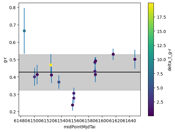
These colours can then be run through the previously written outlier detection functions. We have recorded metadata which can help exclude erroneous colour measurements, such as the time difference between the obs and ref measurements.